M.Eng. Thesis · Harbin Engineering University · 2018 to 2021
PAPR Reduction and Neural Network Distortion Removal for Underwater Acoustic OFDM
Battery powered underwater acoustic modems spend much of their energy in the transmit power amplifier, and
OFDM makes that amplifier inefficient: its peaks sit about 11 dB above the average power, so the amplifier has
to run far below saturation. My M.Eng. thesis attacked the problem from both ends of the link. At the
transmitter I reduced the peak-to-average power ratio (PAPR) with repeated clipping and filtering and a rooting
companding transform, alongside the selected mapping and partial transmit sequence methods from my published
papers. At the receiver I trained a small neural network to learn the power amplifier and removed its
distortion by frequentative decision feedback (FFB). Every result on
this page comes from the open implementation of this work, and the lab runs the same engine live in your browser.
Underwater sensor networks watch the ocean for months at a time on battery power: moored oceanographic
sensors, seabed stations, autonomous vehicles and gliders, environmental monitors and subsea oil and gas
equipment. Radio fades within metres in seawater, so these systems talk with sound, and the power amplifier
that drives the transmitting transducer is one of the largest energy costs in the modem. Every decibel it
wastes shortens how long a deployment can last.
OFDM is the modulation of choice for high rate underwater links because it turns a long, frequency selective
multipath channel into hundreds of narrow subcarriers that are each easy to equalise. Its weakness is the
peak-to-average power ratio: the inverse FFT adds hundreds of subcarriers together, and now and then they line up
into a peak far above the average. The amplifier must stay linear at those peaks, so it spends most of its time
backed off, where it is inefficient. An ideal class B amplifier averages 78.5% efficiency at full drive but only
about 22.3% when backed off by the 10.92 dB an OFDM signal needs.
My goal was a low complexity, energy efficient OFDM system for battery powered underwater modems, and I
worked on both ends of the link:
Transmitter · Chapter 3
Repeated Clipping and Filtering
Clip every peak above a threshold, filter the regrowth out of the band, repeat. I studied how the clipping ratio, oversampling factor and pilot layout trade PAPR against bit error rate for underwater acoustic OFDM.
10.97 to 5.39 dB in four passes
Transmitter · Chapter 3
Rooting Companding
A power law compander |x|R that keeps the phase, with exponents from 0.1 to 0.9 and the inverse applied at the receiver.
R = 0.5: 10.84 to 6.03 dB
Transmitter · Published
Selected Mapping and PTS
Distortionless methods from my published papers: transmit the best of several phase rotated copies of each symbol and send a few bits of side information.
SLM, 16 candidates: 11.15 to 8.03 dB
Receiver · Chapter 4
Neural Network Receiver
A 6-12-6 network learns the power amplifier from measured samples, and frequentative decision feedback uses it to estimate and subtract the amplifier's distortion.
48x fewer bit errors at 3 dB back-off
Figure 1. The link I studied. Amber blocks are where PAPR is created or reduced, blue is the ocean channel, green is the receiver side distortion removal.
Results at a glance
5.58 dB
PAPR removed by four clip and filter passes
42.2%
Ideal class B efficiency, up from 22.2%
48x
Fewer bit errors with FFB at 3 dB back-off
55.6%
Amplifier efficiency at the back-off FFB allows
22
Unit tests behind these numbers
Interactive Lab
The Transmitter view generates random OFDM symbols and applies the method
you pick; the PAPR distribution, amplifier efficiency, distortion and spectrum update as symbols accumulate. The
Receiver view runs the whole link, amplifier, channel, noise and FFB, with
the neural network weights trained in Python. The Channel view shows the
BELLHOP multipath and the guard interval it calls for.
Loading the lab…
OFDM Peaks and How They Are Measured
An OFDM symbol is the inverse FFT of N data symbols Xk. When N is large, the time samples behave like
complex Gaussian noise, so their power follows an exponential distribution and a few samples are much stronger
than the rest. The PAPR of one symbol is its peak sample power over its mean power, and because it changes from
symbol to symbol it is reported as a complementary cumulative distribution function (CCDF), Pr[PAPR > z].
Every PAPR on this page is read at CCDF 10-3: the level exceeded by one symbol in a thousand.
The closed form treats the N Nyquist rate samples as independent. The transmitted analogue signal peaks
between those samples, so PAPR has to be measured on an oversampled signal: I zero pad the middle of the
spectrum by a factor I before the IFFT, with I = 4 whenever accurate peaks matter.
Chapter 3: 128 subcarriers, QPSKChapter 4: 512 subcarriers in 6.25 kHzFFT 8192 at 100 kHzBand 7.9 to 14.1 kHz around 11 kHz20,000 symbols per curve
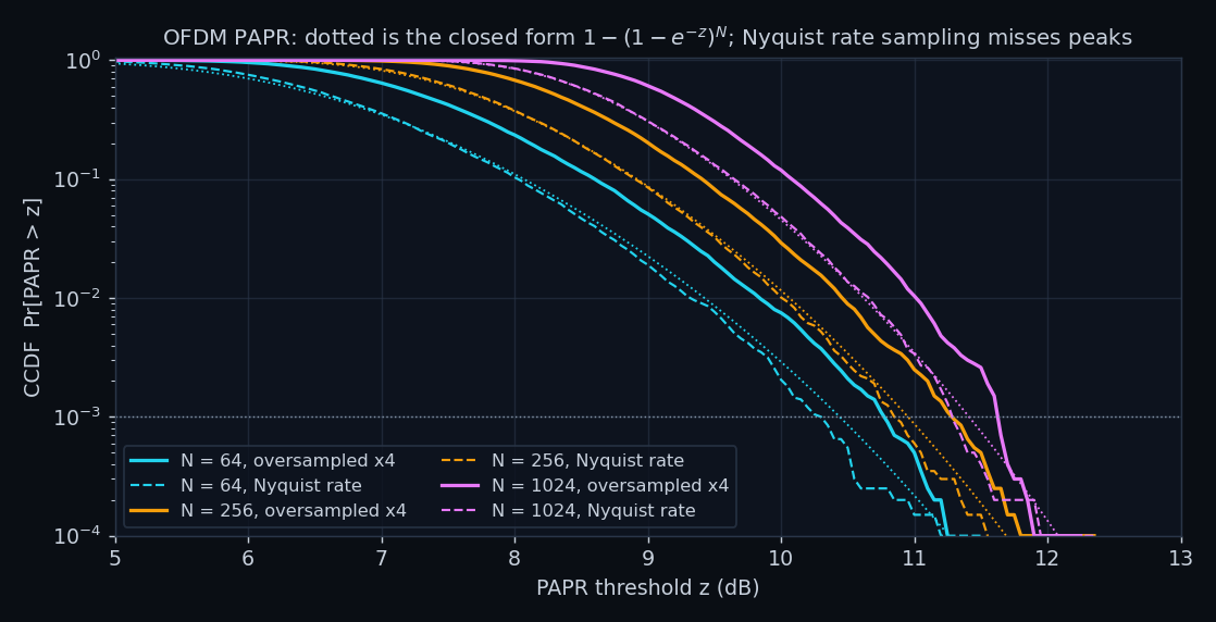
Figure 2. PAPR distribution for three OFDM sizes, oversampled (solid) and at the Nyquist rate (dashed), with the closed form (dotted).
ResultAt CCDF 10-3 the PAPR is 11.03 dB for 128 subcarriers and 11.49 dB for 512,
measured with fourfold oversampling. Sampling at the Nyquist rate underestimates it by 0.34 to
0.48 dB, and at the Nyquist rate the simulation agrees with the closed form to within 0.17 dB
for every size from 64 to 1024.
Why the peaks matter for energy: an amplifier backed off by the PAPR so that its peaks just reach saturation
averages about (π/4)·10−PAPR/20 efficiency if it is an ideal class B stage, and
0.5·10−PAPR/10 for class A. Real amplifiers do worse, but the scaling holds: every decibel
of PAPR removed lets the same battery radiate the same power for longer. I use the class B rule as a simple,
comparable figure of merit throughout.
Repeated Clipping and Filtering
Clipping is the simplest way to remove peaks: every sample above a threshold is scaled down to it with its
phase kept. I set the threshold through the clipping ratio CR, the clipping power over the mean power of the
symbol, so the amplitude limit is √(CR·E|x|2). Clipping alone throws energy outside the
band, so repeated clipping and filtering (RCF) follows every clip with a frequency domain filter: FFT, zero the
out-of-band bins, inverse FFT. The filter lets a few peaks grow back, so the clip and filter pair is repeated,
four times here. Armstrong introduced the idea for radio OFDM [1]; my thesis applied it to underwater acoustic
OFDM and mapped its tradeoffs.
128 subcarriers, QPSKOversampling I = 2CR = 3 (4.77 dB)1 to 4 passes20,000 symbols
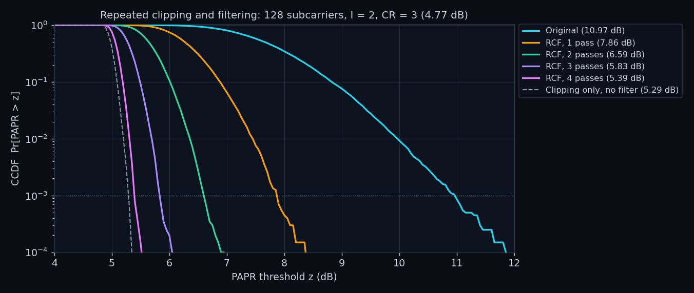
Figure 3. PAPR after one to four clip and filter passes, with a single clip without the filter for comparison.
ResultThe PAPR at CCDF 10-3 falls from 10.97 dB to 7.86, 6.59, 5.83 and
5.39 dB after one to four passes. Four passes remove 5.58 dB of PAPR and lift the ideal class B
efficiency from 22.2% to 42.2%, a factor of 1.90.
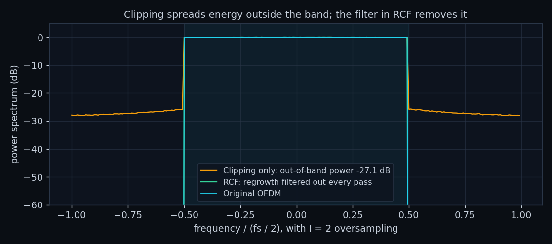
Figure 4. One clip without the filter reaches 5.29 dB PAPR but pushes power out of the band; RCF keeps the spectrum clean.
The cost of RCF is in-band distortion: the clipped energy that stays inside the band adds a noise like error to
every subcarrier, 20.0 dB below the signal for this setting. I measure the price as the extra SNR a QPSK
link needs to reach a bit error rate of 10-4 in white noise; without clipping that SNR is 11.41 dB.
Because the added error is fixed once the data are known, the bit error rate is computed exactly from each bit's
noiseless decision margin rather than by counting errors, which removes Monte Carlo noise from the table.
Table 1: RCF parameter study, four passes, 10,000 symbols per row
Oversampling I
CR (dB)
PAPR at 10-3 (dB)
In-band SDR (dB)
SNR for BER 10-4 (dB)
SNR cost (dB)
1
4 (6.02)
6.02
27.3
11.54
0.14
1
3 (4.77)
4.79
21.7
11.92
0.51
1
2 (3.01)
3.12
15.4
13.99
2.58
1
1.75 (2.43)
2.62
13.6
15.91
4.50
1
1.5 (1.76)
2.09
11.8
22.73
11.32
2
4 (6.02)
6.46
25.3
11.62
0.22
2
3 (4.77)
5.41
20.0
12.17
0.76
2
2 (3.01)
4.16
14.2
14.92
3.52
2
1.75 (2.43)
3.86
12.8
17.52
6.11
2
1.5 (1.76)
3.58
11.2
floor above 10-4
∞
4
4 (6.02)
6.87
25.3
11.62
0.22
4
3 (4.77)
5.80
20.0
12.17
0.76
4
2 (3.01)
4.48
14.3
14.88
3.47
4
1.75 (2.43)
4.11
12.8
17.45
6.04
4
1.5 (1.76)
3.73
11.3
floor above 10-4
∞
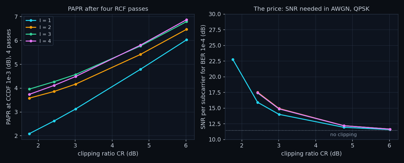
Figure 5. The RCF tradeoff for oversampling I = 1 to 4: PAPR after four passes and the SNR a QPSK link needs for a bit error rate of 10-4.
Reading the tradeoffWith I = 2, CR = 3 cuts the PAPR to 5.41 dB for 0.76 dB more SNR, and CR = 2
reaches 4.16 dB for 3.52 dB. Below CR = 2 the distortion grows faster than the peaks shrink,
and at CR = 1.5 with filtering the bit error rate never reaches 10-4: the clipping itself sets an error
floor. Without the filter (I = 1) the same CR reaches 10-4 at 22.7 dB, at the cost of
out-of-band power.
Rooting Companding
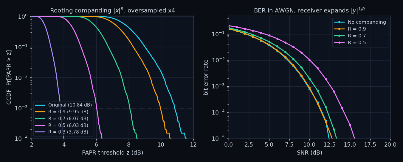
Companding compresses large amplitudes instead of cutting them. My rooting companding transform raises each
sample's amplitude to a power R below one and keeps its phase, f(x) = |x|R·x/|x|, where R = 0.5 is
square root companding and I explored R from 0.1 to 0.9. The receiver restores the amplitudes with
|y|1/R before its FFT. Because the peak amplitude is raised to the same power, the PAPR in dB shrinks
roughly in proportion to R.
Figure 6. Rooting companding for R = 0.3 to 0.9 (left) and the bit error rate when the receiver expands the samples (right).
ResultIn the thesis setting (Nyquist rate, cyclic prefix included) R = 0.5 takes the PAPR from
10.51 dB to 5.85 dB. With fourfold oversampling the original 10.84 dB becomes 9.95,
8.07, 6.03 and 3.78 dB for R = 0.9, 0.7, 0.5 and 0.3. For a bit error rate of 10-4, R = 0.5
needs 14.26 dB of SNR, 2.71 dB more than no companding, because expanding the samples also
stretches the noise.
SpectrumCompanding is a nonlinear operation, so it also spreads power outside
the band. With fourfold oversampling, R = 0.5 sends 1.9% of the transmitted power outside the band
(-17.2 dB), against 0.2% for a single clip, and its in-band distortion sits 15.4 dB below the signal. A practical RCT transmitter
therefore adds a band limiting filter, the same compromise RCF makes explicitly.
Selected Mapping and Partial Transmit Sequences
Distortion based methods change the signal; SLM and PTS only choose among equivalent versions of it. SLM
multiplies the data by U different phase sequences drawn from {±1, ±j}, computes U inverse FFTs and
transmits the candidate with the lowest PAPR, sending log2U bits of side information so the receiver can
undo the rotation [12]. PTS splits the subcarriers into V adjacent blocks, computes one inverse FFT per block, and
searches the WV−1 combinations of block phase factors for the lowest peak, costing
(V−1)·log2W side information bits [13, 14]. Neither adds distortion; both spend computation
and a little rate.
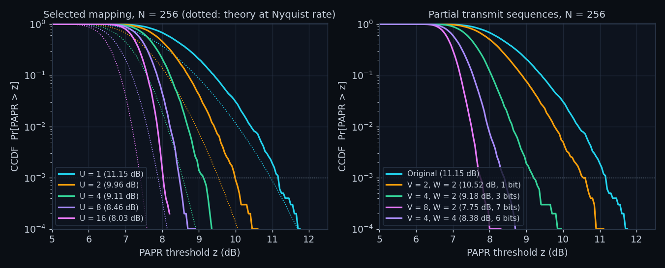
Figure 7. SLM against the closed form (left) and PTS for four block and phase settings (right), 256 subcarriers, 10,000 symbols.
ResultSLM with U = 16 lowers the PAPR from 11.15 dB to 8.03 dB (3.12 dB) for 4
side bits, and at the Nyquist rate the simulation matches the closed form (1 − (1 − e−z)N)U
to within 0.06 dB for every U. PTS reaches 9.18 dB with 4 blocks and 7.75 dB with 8 blocks and two
phase factors, and 8.38 dB with 4 blocks and four phase factors.
Table 2: every method on one footing, 128 subcarriers, fourfold oversampling, QPSK
Method
PAPR at 10-3 (dB)
In-band SDR (dB)
Out-of-band power (dB)
Side information (bits)
FFT work per symbol
Class B efficiency
Original OFDM
10.92
none
none
0
1
22.3% (1.00x)
Clipping only (CR 3)
5.29
25.0
-27.0
0
1
42.7% (1.91x)
RCF (CR 3, 4 passes)
5.82
20.0
none
0
9
40.2% (1.80x)
Rooting companding (R 0.5)
6.06
15.4
-17.2
0
1
39.1% (1.75x)
SLM (U 16)
7.55
none
none
4
16
32.9% (1.47x)
PTS (V 8, W 2)
7.26
none
none
7
8
34.1% (1.53x)
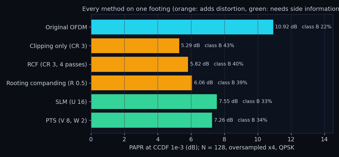
Figure 8. The PAPR each method reaches, with the ideal class B amplifier efficiency it allows.
The table is the design space in one view. Clipping and RCF remove the most PAPR for the least computation
but add distortion; rooting companding is cheap but spreads the spectrum; SLM and PTS are clean but need side
information and several inverse FFTs per symbol. A battery powered modem that can afford a little distortion gets
the most from RCF, and that distortion is exactly what the receiver side of my thesis removes.
Receiver: Learning the Amplifier and Removing Its Distortion
Transmitter methods reduce the peaks, but a real amplifier still compresses whatever peaks remain, and the
cheaper and more efficient the amplifier, the harder it compresses. My idea was to leave the amplifier alone and
clean up its distortion at the receiver, where computation is less constrained than in a battery powered
transmitter.
The amplifier
I model the transmit amplifier as a solid state power amplifier (Rapp model, smoothness p = 2), which
compresses amplitude and leaves phase alone. Its drive is set by the input back-off, how far the saturation level
sits above the RMS input amplitude, and I evaluate 3, 5 and 7 dB. By Bussgang's theorem the output is a scaled copy
of the input plus a distortion term uncorrelated with it, y = αx + d, and that distortion d is what the
receiver has to remove.
The network
The receiver does not know the amplifier's equations, so it learns them. The time signal's amplitudes are
reshaped into vectors of six consecutive samples, one hidden layer of 12 sigmoid neurons maps them to six output
amplitudes (162 weights in total), and the network is trained with the Levenberg-Marquardt algorithm [9] on 25,800
amplifier samples measured at 35 dB SNR, split randomly 70/15/15 with validation based early stopping.
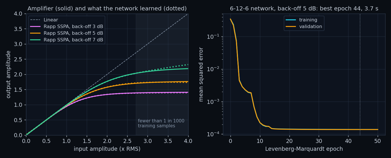
Figure 9. The amplifier at three back-off levels and what the network learned (left); training history at 5 dB back-off (right).
ResultAt 5 dB back-off training stops at epoch 44 after 3.7 s with a validation MSE of
1.4×10⁻⁴ and a test MSE of 1.4×10⁻⁴. Up to three times the RMS amplitude the learned curve stays within
0.054 of the true one at every back-off, and the Bussgang gain it implies, 0.9147, matches the exact
0.9146. Each output depends on its own input: nudging a neighbouring input moves it by at most
2.2% as much, so the network has correctly learned that the amplifier has no memory.
The channel
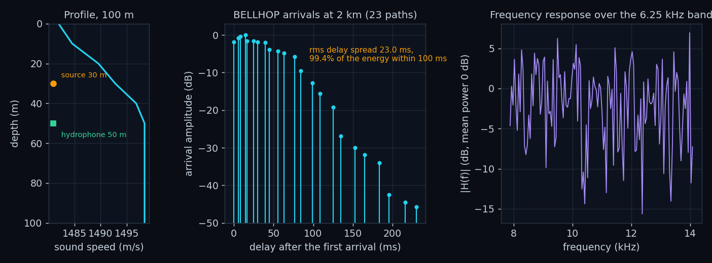
The channel is a BELLHOP ray tracing model of the chapter 4 link: 100 m of water, the transmitter at 30 m and
the hydrophone at 50 m, 2 km apart, at 11 kHz, with the sound speed rising from 1482 m/s at the surface to 1498.4 m/s
at 50 m over a sandy bottom. The arrivals are read with the parser I validated in my BELLHOP report.
Figure 10. Sound speed profile and geometry, the 23 BELLHOP arrivals at 2 km, and the resulting frequency response across the band.
Physical checkThe first arrival reaches the hydrophone after 1.3374 s; the straight line distance at the
harmonic mean sound speed predicts 1.3368 s, a difference of 0.048%. Across the band the response swings
from -26.3 dB to about +7 dB, with 7.6% of the subcarriers faded by more than 10 dB.
Guard intervalThe channel's rms delay spread is 23.0 ms, its last arrival comes 230 ms after
the first, and 99.4% of its energy lands within 100 ms. The link model gives each subcarrier the channel's
frequency response (thesis equation 4-18), which holds when the guard interval covers the multipath; the Channel
view of the lab shows how the energy outside the guard falls as the guard grows, and what that costs in airtime.
Frequentative decision feedback
The received subcarriers are Yk = Hk(αXk + Dk) + Wk,
where Dk is the FFT of the amplifier distortion. D depends on the whole transmitted symbol, so the
receiver cannot compute it until it knows the symbol, and it cannot know the symbol reliably until D is removed.
FFB breaks the circle by iterating, the approach Tellado, Hoo and Cioffi [7] and Chen and Haimovich [8] took for
known clipping; my contribution was to let a learned model stand in for the amplifier, so the receiver never needs
the amplifier's equations:
Equalise with the known channel: Zk = Yk / Hk, and start with D = 0.
Decide: X̂k is the nearest QAM point to (Zk − Dk) / α.
Reconstruct the transmitted signal from the decisions: x̂ = IFFT(X̂), oversampled four times.
Run it through the learned amplifier: ŷ = network(|x̂|), with the phase of x̂.
Estimate the distortion, D = FFT(ŷ − αx̂) on the in-band bins, and return to step 2.
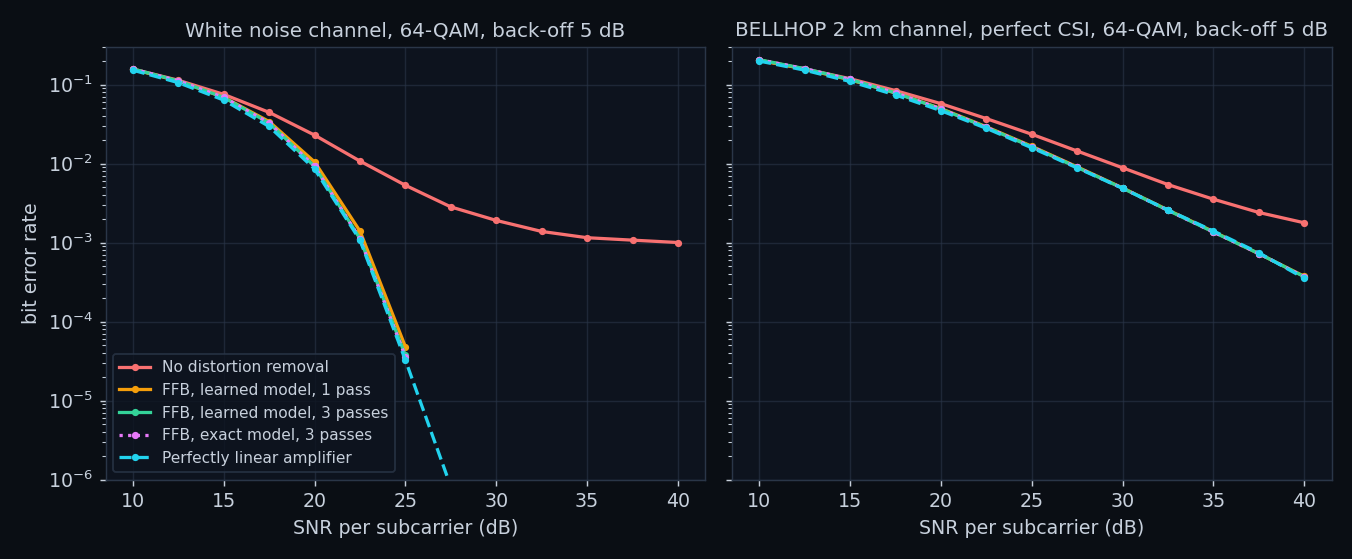
Figure 11. 64-QAM at 5 dB back-off: without distortion removal, with FFB using the learned network (one and three passes) and the exact amplifier, and a perfectly linear amplifier for reference. 400 symbols (1,228,800 bits) per point.
ResultIn white noise the amplifier alone leaves an error floor of 1.0×10⁻³ at 40 dB SNR; one FFB pass
with the learned network removes it, and after three passes the link needs 22.59 dB for a bit error rate of
10-3, against 22.55 dB for a perfectly linear amplifier. Over the BELLHOP channel the floor of
1.8×10⁻³ at 40 dB falls to 3.7×10⁻⁴ with the learned network and 3.7×10⁻⁴ with the exact equations; the
linear amplifier gives 3.5×10⁻⁴. The learned network performs as well as knowing the amplifier exactly.
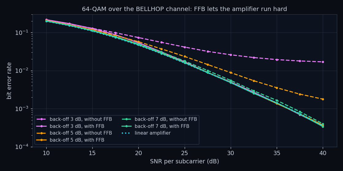
Figure 12. 64-QAM over the BELLHOP channel at three amplifier back-off levels, with and without FFB.
What FFB buys the batteryAt 3 dB back-off the amplifier alone leaves 1.7×10⁻² of the bits wrong at
40 dB SNR; FFB brings that to 3.5×10⁻⁴, 48 times fewer errors and level with a linear amplifier
(3.5×10⁻⁴). Of the 3, 5 and 7 dB back-off levels, only 7 dB lets this link reach a bit error rate of 10-3
without FFB (36.8 dB SNR); with FFB it gets there at 3 dB back-off (36.2 dB, against 36.3 dB
for a linear amplifier). An ideal class B amplifier averages 55.6% efficiency at 3 dB back-off and 35.1% at 7 dB,
so for the same radiated power it draws 1.58 times less from the battery. A clipper ahead of the
amplifier behaves the same way: 4.9×10⁻³ without FFB and 3.8×10⁻⁴ with it at 40 dB.
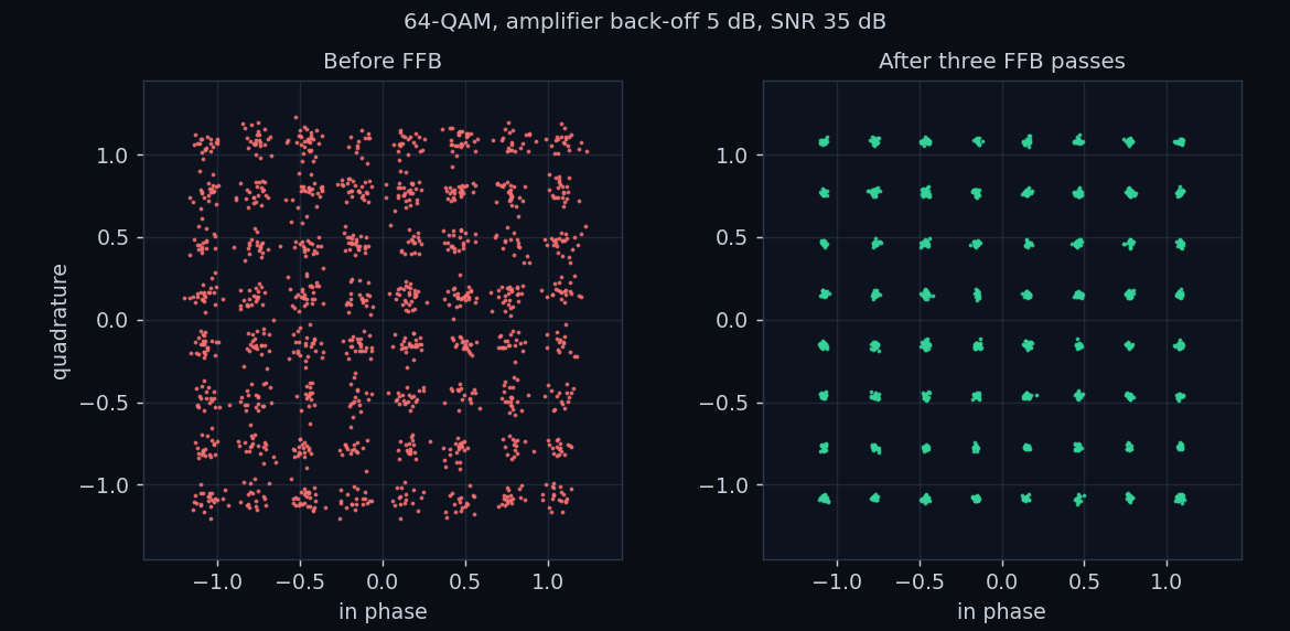
Figure 13. 64-QAM at 5 dB back-off and 35 dB SNR, before and after three FFB passes.
Over the BELLHOP channel FFB recovers linear amplifier performance and no more: what remains is set by the
subcarriers sitting in deep fades, which only channel coding or diversity can fix. That is the natural limit of
receiver side distortion removal, and it is why the white noise and channel results are shown side by side.
Applications
Ocean observation
Long-term Sensor Networks
Moored and seabed networks that report temperature, currents, acoustics or water quality for months. Energy per bit sets how long a deployment lasts, and lower PAPR plus receiver side cleanup lets the same battery carry more data.
Autonomy
Vehicles and Gliders
AUV and glider telemetry and command links, where every watt spent on the acoustic modem is a watt not spent on propulsion or sensing.
Offshore
Energy and Infrastructure
Wireless monitoring of subsea oil and gas equipment, pipelines and offshore wind foundations, where cables are expensive and divers are dangerous.
Safety
Early Warning and Security
Tsunami and seabed pressure buoys, harbour and coastal surveillance, and naval sensor networks that must run unattended.
Radio
4G, 5G, Wi-Fi and Satellite
The same peak problem shapes 4G and 5G (it is why the LTE uplink uses single carrier FDMA), Wi-Fi, digital television and satellite links; clipping and filtering and neural network amplifier models are standard tools there.
Next steps
Where the Work Went
A long short-term memory network for PAPR reduction in underwater OFDM (JASA 2021 [16], KSII Transactions 2023 [17]), and co-authored deep learning OFDM receivers [18, 19].
Code and Reproducibility
This work is open source at github.com/raza-waleed/underwater-acoustic-ofdm-papr-reduction:
a numpy package for the OFDM model, the PAPR methods, the amplifier, the BELLHOP channel, the neural network and the
FFB receiver, together with the experiment and figure scripts, the browser lab and the tests.
How the numbers are protected22 unit tests pin the claims on this page, including exact inverses, SLM
against its closed form, PTS against brute force, the BELLHOP geometry check, and FFB removing every noiseless
distortion error. The lab's JavaScript engine recomputes nine reference cases exported by Python on every page load,
and every number on this page is filled in from the experiment output by the build script, which refuses to build
if one is missing.
pip install -r requirements.txt
python experiments/run_all.py        # every experiment, about 5 minutes
python experiments/make_figures.py   # the figures
python build.py                      # this page
python -m unittest discover -s tests
State the measurement with the number. A PAPR means little without its CCDF level and sampling
rate, and an SNR means little without saying where it was measured; every number on this page carries both.
Distortion moves; it does not vanish. Clipping trades peaks for in-band error and spectrum, RCF
trades the spectrum back for computation, rooting companding trades peaks for noise enhancement, and SLM and PTS
trade them for side information. The useful question is always which resource the system can spare.
A receiver can clean up the amplifier, not the ocean. FFB with a 162 weight network matches a
linear amplifier, which means the transmitter can run its amplifier much harder; beyond that point the fading
channel sets the error rate, and the next gains come from coding and diversity.
Size the waveform from the channel. The BELLHOP channel spreads its energy over tens of
milliseconds, which sets the guard interval and the symbol length, the same lesson my lake trial report drew from its
measured coherence time.
Nomenclature and References
AWGNadditive white Gaussian noise
BERbit error rate
CCDFcomplementary cumulative distribution function
CRclipping ratio (clipping over mean power)
FFBfrequentative decision feedback
Ioversampling factor
OFDMorthogonal frequency division multiplexing
PAPRpeak-to-average power ratio
PTSpartial transmit sequences
QAMquadrature amplitude modulation
RCFrepeated clipping and filtering
RCTrooting companding transform
SDRsignal to distortion ratio
SLMselected mapping
SNRsignal to noise ratio
SSPAsolid state power amplifier
References
[1] J. Armstrong, "Peak-to-average power reduction for OFDM by repeated clipping and frequency domain filtering," Electronics Letters, vol. 38, no. 5, pp. 246-247, 2002.
[2] R. W. Bäuml, R. F. H. Fischer and J. B. Huber, "Reducing the peak-to-average power ratio of multicarrier modulation by selected mapping," Electronics Letters, vol. 32, no. 22, pp. 2056-2057, 1996.
[3] S. H. Müller and J. B. Huber, "OFDM with reduced peak-to-average power ratio by optimum combination of partial transmit sequences," Electronics Letters, vol. 33, no. 5, pp. 368-369, 1997.
[4] X. Wang, T. T. Tjhung and C. S. Ng, "Reduction of peak-to-average power ratio of OFDM system using a companding technique," IEEE Transactions on Broadcasting, vol. 45, no. 3, pp. 303-307, 1999.
[5] R. van Nee and A. de Wild, "Reducing the peak-to-average power ratio of OFDM," Proc. IEEE Vehicular Technology Conference, 1998, pp. 2072-2076.
[6] C. Rapp, "Effects of HPA-nonlinearity on a 4-DPSK/OFDM-signal for a digital sound broadcasting system," Proc. Second European Conference on Satellite Communications, 1991, pp. 179-184.
[7] J. Tellado, L. M. C. Hoo and J. M. Cioffi, "Maximum-likelihood detection of nonlinearly distorted multicarrier symbols by iterative decoding," IEEE Transactions on Communications, vol. 51, no. 2, pp. 218-228, 2003.
[8] H. Chen and A. M. Haimovich, "Iterative estimation and cancellation of clipping noise for OFDM signals," IEEE Communications Letters, vol. 7, no. 7, pp. 305-307, 2003.
[9] M. T. Hagan and M. B. Menhaj, "Training feedforward networks with the Marquardt algorithm," IEEE Transactions on Neural Networks, vol. 5, no. 6, pp. 989-993, 1994.
[10] M. B. Porter, The BELLHOP Manual and User's Guide, Heat, Light, and Sound Research, 2011.
[11] X. Ma, W. Raza, Z. Wu, M. Bilal, Z. Zhou and A. Ali, "A nonlinear distortion removal based on deep neural network for underwater acoustic OFDM communication with the mitigation of peak to average power ratio," Applied Sciences, vol. 10, no. 14, 4986, 2020.
[12] W. Raza, X. Ma, A. Ali, A. Raza and S. Shaikh, "Performance analysis of selective mapping in underwater acoustic orthogonal frequency division multiplexing communication system," Engineering, Technology & Applied Science Research, vol. 11, no. 1, pp. 6696-6702, 2021.
[13] W. Raza, X. Ma, T. Wang and M. Bilal, "Low complexity energy efficient OFDM communication system over underwater acoustic channel by partial transmit sequence peak to average power ratio reduction," J. Acoust. Soc. Am., vol. 146, no. 4, pp. 2764-2765, 2019.
[14] W. Raza, X. Ma, A. Ali, Z. A. Shah and G. Mehdi, "An implementation of partial transmit sequences to design energy efficient underwater acoustic OFDM communication system," arXiv:2007.01273, 2020.
[15] W. Raza, "PAPR reduction with nonlinear distortion removal using machine learning in underwater acoustic OFDM communication system," M.Eng. thesis, Harbin Engineering University, 2021.
[16] W. Raza, X. Ma and M. Bilal, "Long short-term memory neural network assisted peak to average power ratio reduction for underwater acoustic OFDM communication," J. Acoust. Soc. Am., vol. 150, p. A319, 2021.
[17] W. Raza, X. Ma, H. Song, A. Ali, H. Zubairi and K. Acharya, "Long short-term memory neural network assisted peak to average power ratio reduction for underwater acoustic OFDM communication," KSII Transactions on Internet and Information Systems, vol. 17, 2023.
[18] A. Ali, B. Chen, W. Raza, A. H. Samo and A. Ali, "Reduction of PAPR by convolutional neural network with soft feedback in an underwater acoustic OFDM communication," Proc. 18th International Bhurban Conference on Applied Sciences and Technology, 2021.
[19] A. Ali, B. Chen, W. Raza, A. H. Samo and A. Ali, "Deep learning based OFDM system for underwater acoustic communication with mitigation of peak to average power ratio," International Journal of Scientific & Technology Research, vol. 9, no. 12, pp. 117-122, 2020.
Materials. The code, experiments, tests, figures, browser lab, and the BELLHOP input and arrivals output
for this work are in the repository. BELLHOP itself is Michael B. Porter's Acoustics Toolbox and is cited, not
redistributed. The thesis document is summarised here and not published.