Underwater Acoustic Transducer & Hydrophone Systems: Architecture, Characterization, and Computational Modeling
List of Figures (23)
- Figure 1: End-to-end transmit/receive signal chain
- Figure 2: Tonpilz transducer cross-section
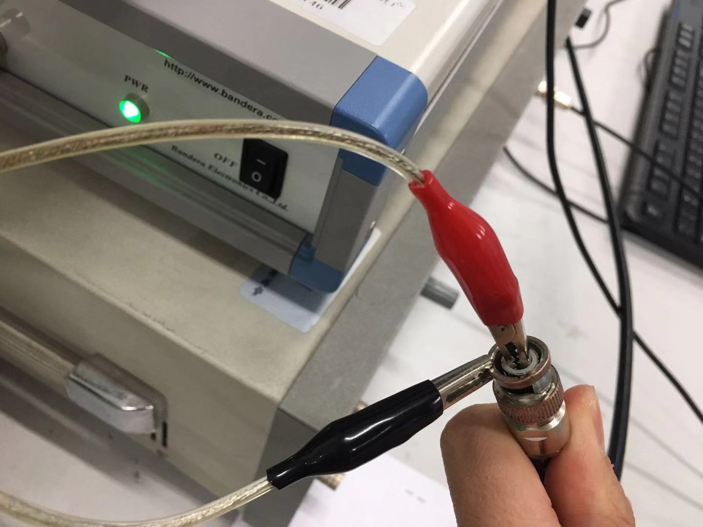
- Figure 3: Impedance measurement setup photograph
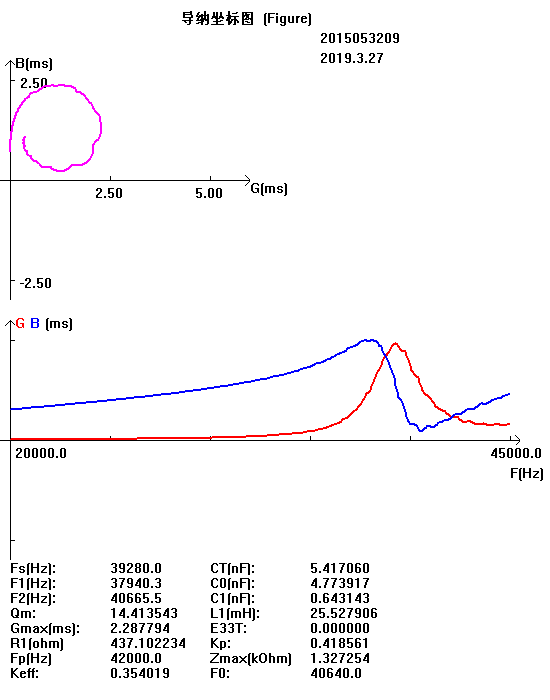
- Figure 4: Hydrophone admittance circle and G/B, in air
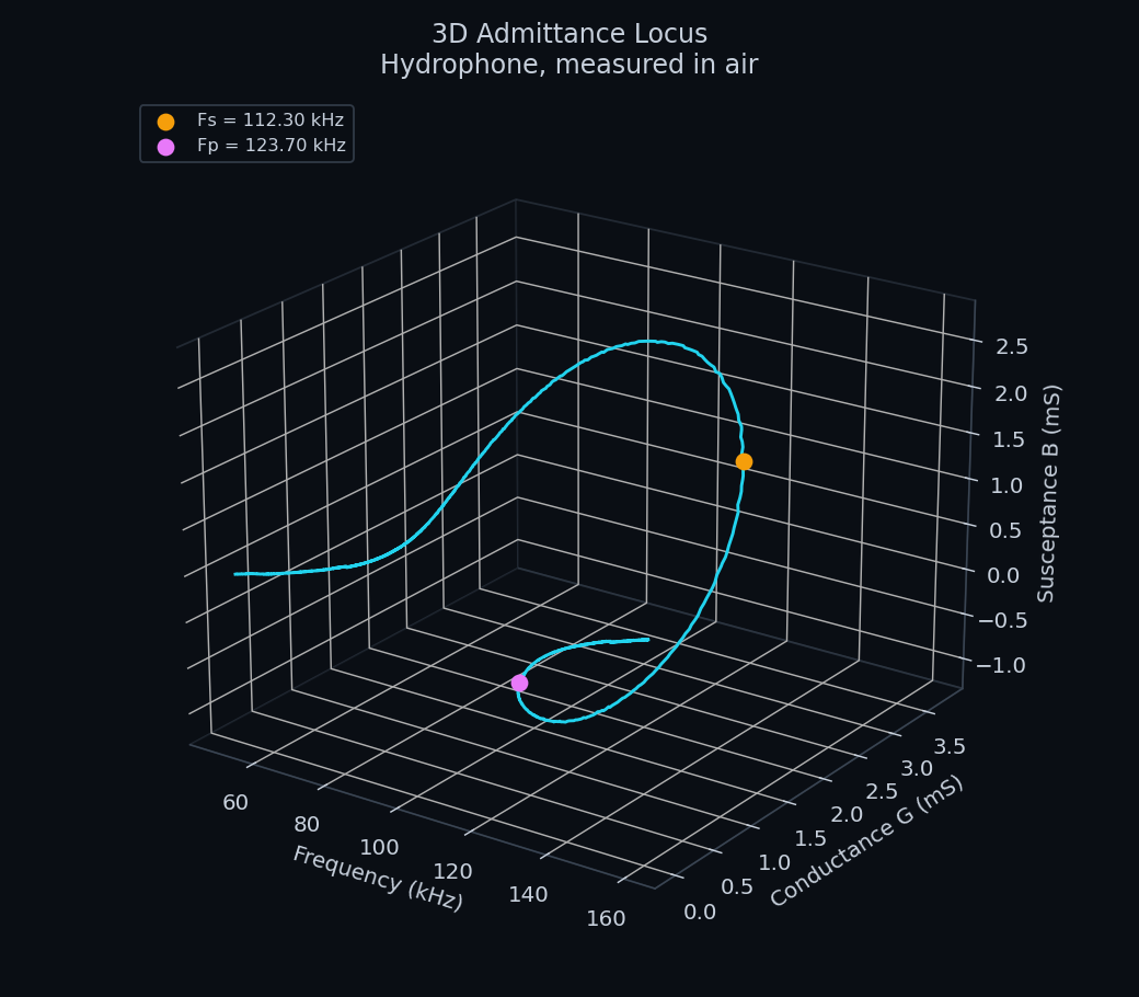
- Figure 5: Hydrophone admittance locus in 3D, in air
- Figure 6: Hydrophone admittance circle and G/B, in water
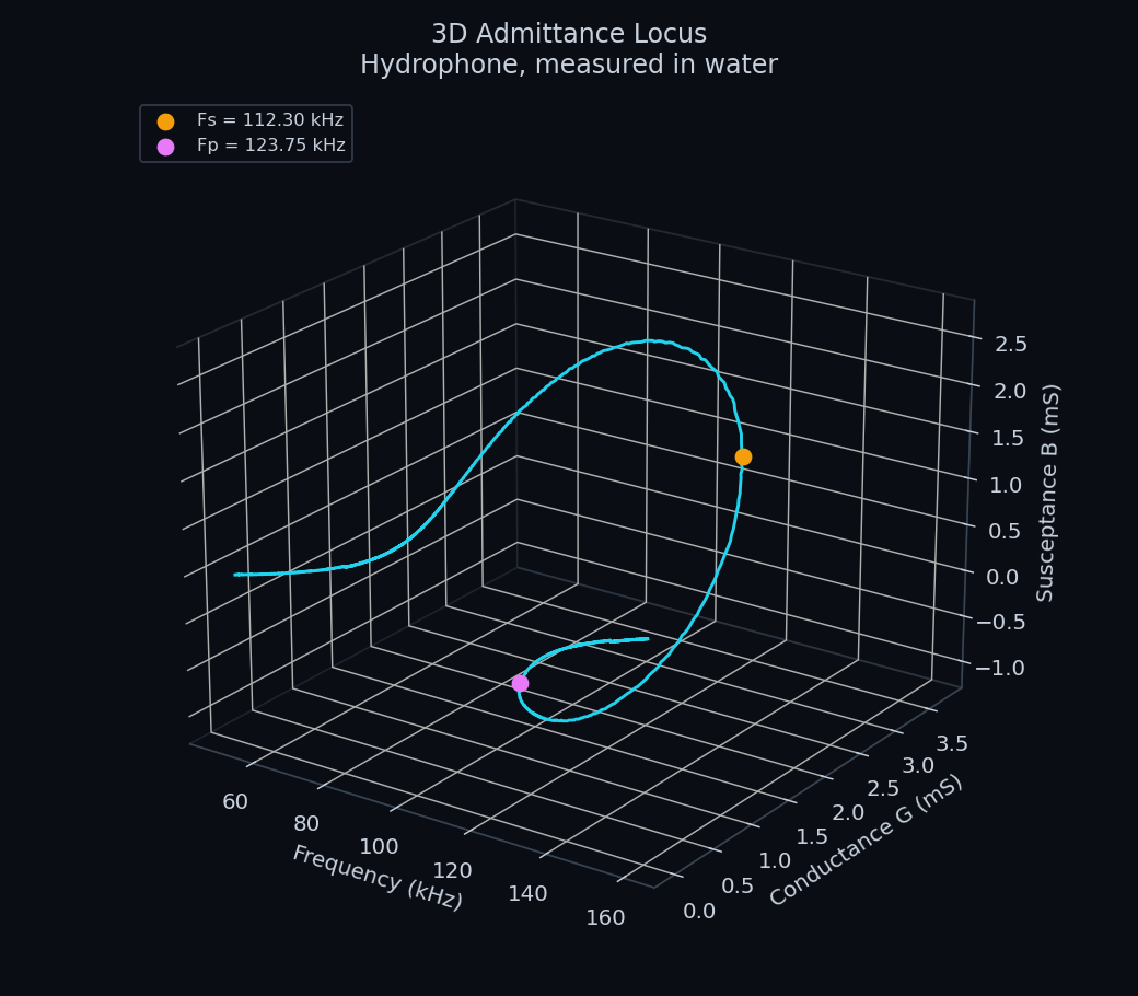
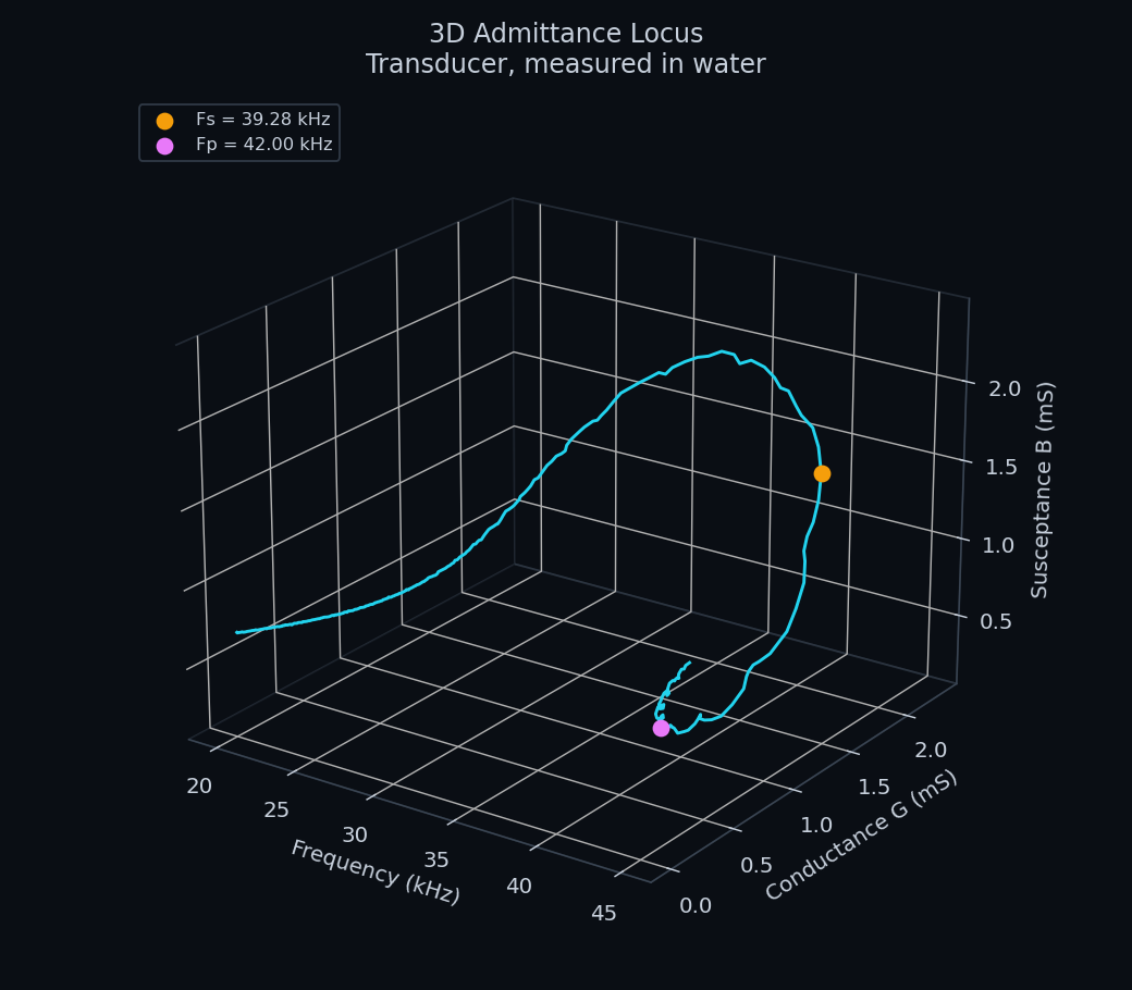
- Figure 7: Hydrophone admittance locus in 3D, in water
- Figure 8: Transducer admittance circle and G/B, in air
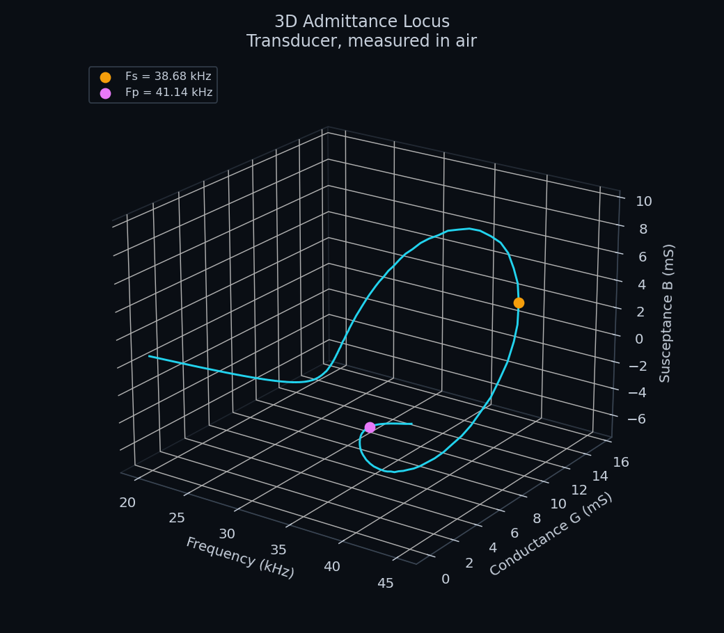
- Figure 9: Transducer admittance locus in 3D, in air
- Figure 10: Transducer admittance circle and G/B, in water
- Figure 11: Transducer admittance locus in 3D, in water
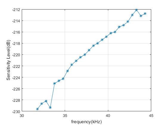
- Figure 12: Free-field sensitivity level versus frequency
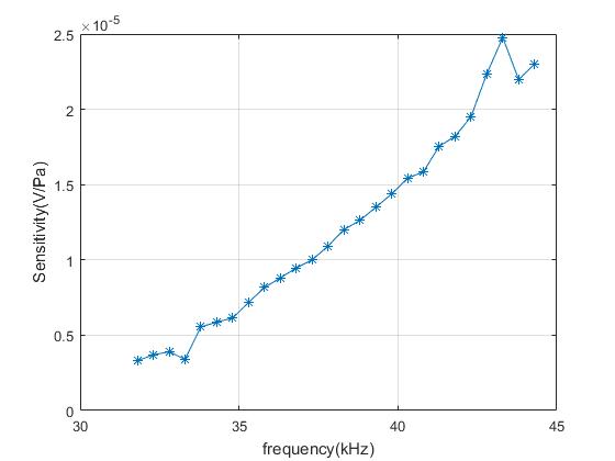
- Figure 13: Free-field sensitivity in V/Pa versus frequency
- Figure 14: Measured TVR versus frequency
- Figure 15: TVR beam map in 3D
- Figure 16: Measured directivity, linear scale
- Figure 17: Measured directivity, dB scale
- Figure 18: Measured directivity reconstructed in 3D
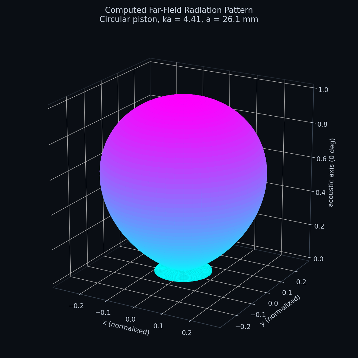
- Figure 19: Computed 3D far-field radiation pattern
- Figure 20: Polar comparison, modeled vs. measured
- Figure 21: FFT magnitude spectrum, 5 kHz record
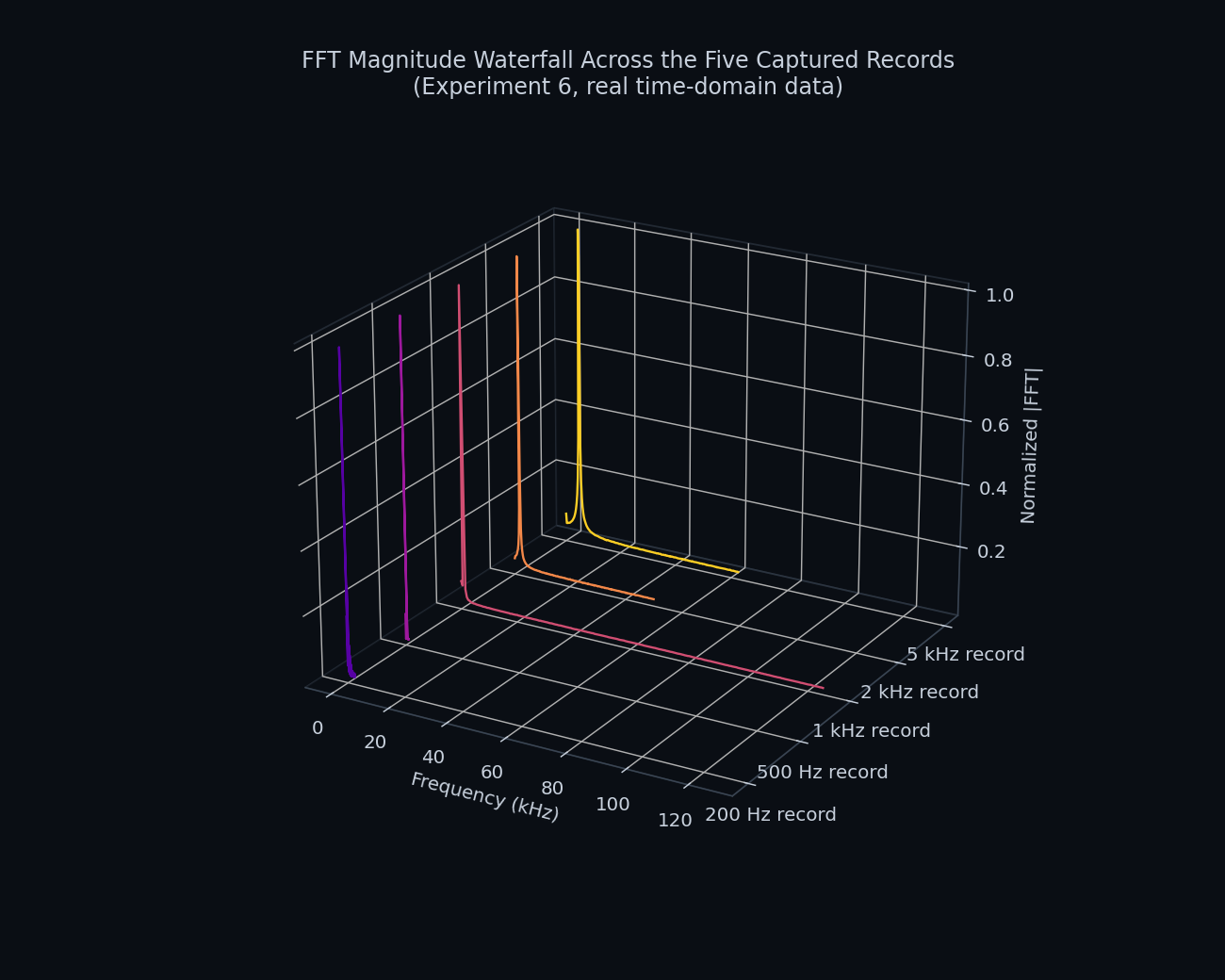
- Figure 22: FFT magnitude waterfall across five records
1. System Architecture & Signal Chain
An underwater acoustic measurement system separates cleanly into a transmit (TX) chain that generates and radiates an acoustic signal into the water, and a receive (RX) chain that captures the propagated signal and converts it back to an analyzable electrical waveform. Every measurement in this report, including impedance, sensitivity, transmitting response, and directivity, is a variation on driving this same signal chain and analyzing what comes back, as laid out in Figure 1.
2. Transducer Construction & Operating Principle
An electroacoustic transducer converts electrical energy into acoustic energy (acting as a projector) or acoustic energy into electrical energy (acting as a hydrophone); many devices are reciprocal and can perform both roles. The dominant mechanism in modern underwater transducers is the piezoelectric effect: an applied electric field induces mechanical strain in a piezoceramic (commonly lead zirconate titanate, PZT), and conversely, mechanical stress on the ceramic generates a proportional electrical charge. The most widely used low-frequency sonar transducer architecture built on this effect is the Tonpilz ("sound mushroom") design, illustrated in Figure 2 below.
The lightweight head mass couples most of the vibration into the water (impedance-matched to the medium), while the heavy tail mass reflects vibrational energy forward rather than into the mounting structure. A central prestress bolt holds the ceramic stack under permanent compression, since PZT ceramics are strong in compression but weak in tension, which matters most at the high drive levels used in sonar projectors. The whole assembly resonates at a half-wavelength mode set by the head/tail mass ratio, giving the transducer its characteristic resonant frequency and radiation efficiency.
3. Electrical Impedance Characterization
A piezoelectric transducer's electrical impedance traces a characteristic resonance/antiresonance pair at its mechanical resonant frequency; loading the front face with water (a much higher acoustic impedance than air) damps and shifts this resonance, which is exactly the mechanism used here to distinguish the transducer's in-air and in-water electromechanical behavior. The device under test was connected to the impedance analyzer by a pair of alligator clips onto a BNC connector, shown in Figure 3, and impedance curves were acquired via the analyzer's own dedicated measurement software, exported as raw frequency, conductance (G), and susceptance (B) triples, and cross-validated against an independent MATLAB re-plot of the same raw data. The resulting admittance circle and conductance/susceptance curves for the hydrophone and for the transducer, each measured in air and in water, appear in Figures 4, 6, 8, and 10.
Measurement setup
Measured impedance curves
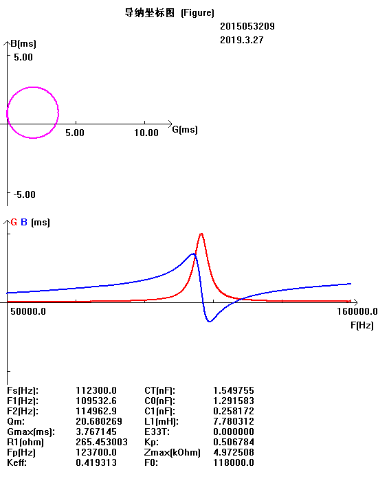
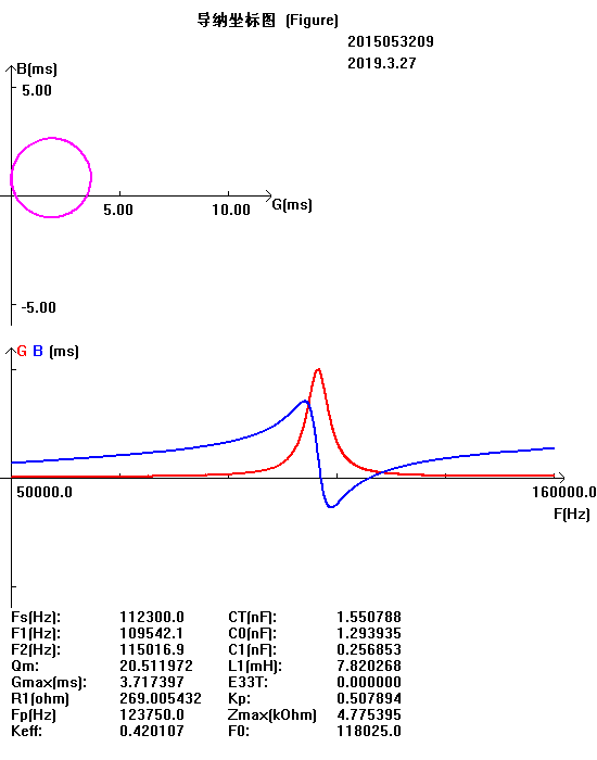
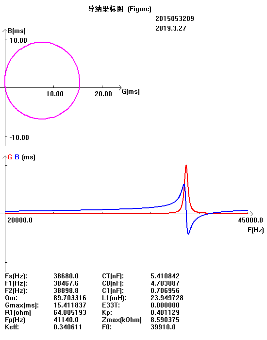
The admittance circle and the G/B-versus-frequency curves above are two 2D projections of one underlying relationship: conductance and susceptance are both functions of frequency at the same time. Figures 5, 7, 9, and 11 plot that relationship directly, as a single parametric curve through frequency, conductance, and susceptance space, built from the same raw exported data (not the screenshots, the underlying frequency/G/B records behind them). The series resonance Fs is marked where conductance peaks, and the antiresonance Fp is marked at the local minimum of admittance magnitude beyond Fs. These two frequencies are exactly what Section 7 uses to compute the electromechanical coupling coefficient for each condition.
4. Free-Field Voltage Sensitivity
Hydrophone sensitivity, defined as the ratio of open-circuit output voltage to the incident free-field sound pressure, was determined by the comparison calibration method: a standard (pre-calibrated) reference hydrophone and the test hydrophone are exposed to the same acoustic field in turn, and the test unit's sensitivity is derived from the ratio of their outputs. The frequency sweep below was captured at a fixed drive level and geometry so that pressure at the receiver stayed constant across frequency, and is presented as sensitivity level in Figure 12 and as sensitivity in volts per pascal in Figure 13.
Output electric signal of the standard hydrophone
| Frequency (kHz) | Voltage / grid | # grids |
|---|---|---|
| 44.3 | 3.60 | 30 |
| 43.8 | 3.44 | 30 |
| 43.3 | 4.00 | 30 |
| 42.8 | 3.84 | 30 |
| 42.3 | 3.84 | 30 |
| 41.8 | 4.32 | 30 |
| 41.3 | 4.96 | 30 |
| 40.8 | 5.36 | 30 |
| 40.3 | 5.76 | 30 |
| 39.8 | 6.24 | 30 |
| 39.3 | 6.40 | 30 |
| 38.8 | 6.24 | 30 |
| 38.3 | 5.76 | 30 |
| 37.8 | 4.96 | 30 |
| 37.3 | 4.24 | 30 |
| 36.8 | 3.68 | 30 |
| 36.3 | 3.20 | 30 |
| 35.8 | 2.72 | 30 |
| 35.3 | 2.32 | 30 |
| 34.8 | 1.92 | 30 |
| 34.3 | 1.84 | 30 |
| 33.8 | 1.68 | 30 |
| 33.3 | 1.03 | 30 |
| 32.8 | 1.18 | 30 |
| 32.3 | 1.12 | 30 |
| 31.8 | 1.00 | 30 |
Peak response at 39.3 to 39.8 kHz identifies the transducer's mechanical resonance, consistent with the 39.8 kHz working frequency used for the transmitting response and directivity measurements in Section 5.
Figures
5. Transmitting Voltage Response & Directivity
5.1 Transmitting Voltage Response (TVR)
The Transmitting Voltage Response, defined as the ratio of the far-field acoustic pressure produced (referred to 1 m) to the drive voltage applied, was measured against the standard reference hydrophone under the comparison method, then plotted as a frequency response curve, shown in Figure 14.
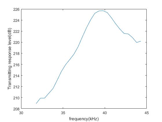
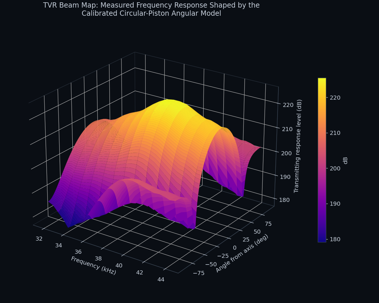
To see how this frequency response combines with the transducer's angular directivity, Figure 15 reshapes the same measured curve into a three dimensional beam map. The on-axis level at each frequency is the real transmitting response data plotted in Figure 14, and the angular roll-off at each frequency comes from the calibrated circular-piston model of Section 5.3, evaluated at that frequency's own value of ka. No new measurement was taken to build this figure; it is a synthesis of two measurements already in this report, and it makes visible something the one-dimensional curve alone cannot: the main lobe narrows visibly as frequency rises through the 39 to 40 kHz resonance, exactly as diffraction theory predicts for a fixed-radius piston. The peak level (225.7 dB at 39.8 kHz) and the −3 dB bandwidth of this curve (3.0 kHz, from 38.3 to 41.3 kHz) are carried forward into the bandwidth discussion in Section 7.3.
5.2 Measured Directivity Pattern
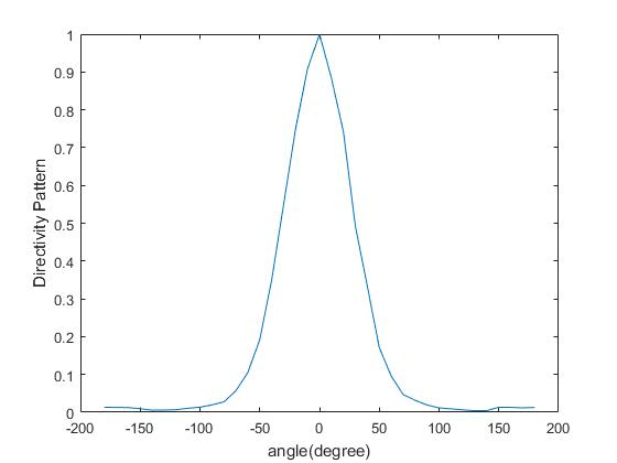
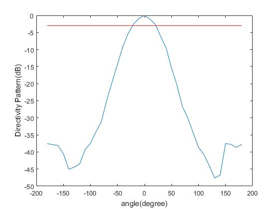
The transmitting transducer's directivity was mapped by rotating it from 0° to 360° in 10° steps at its 39.8 kHz resonance, with the receiving hydrophone fixed 20 cm away and driven by a continuous wave signal through the power amplifier. The resulting pattern is plotted on a linear scale in Figure 16 and on a decibel scale, with the −3 dB line marked, in Figure 17.
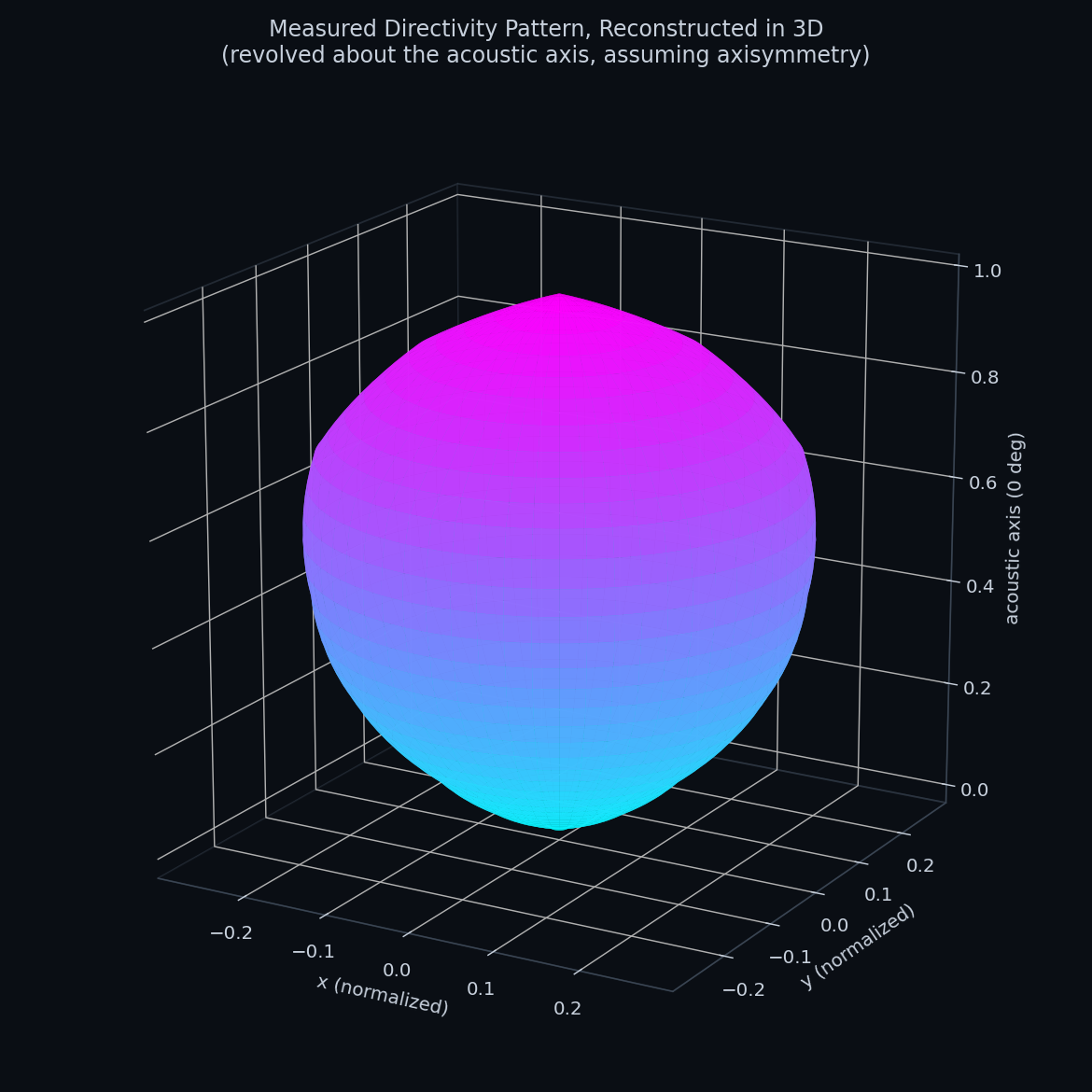
The measurement above is a single cut through the pattern, taken as the transducer was rotated through one full turn in a single plane. Because the transducer's radiating face is circular and the Tonpilz architecture described in Section 2 is axisymmetric about that face, the same profile should hold at every azimuth around the acoustic axis. Figure 18 tests that assumption directly on the real data: it averages the two measured half-turns at each polar angle and revolves the resulting profile a full 360° around the axis, producing a three dimensional reconstruction of the actual measured lobe rather than a theoretical one. The forward lobe dominates while the sides and rear stay close to the noise floor, which is the expected shape for a baffled circular piston and matches the independently derived theoretical model in Section 5.3.
5.3 Computational Radiation-Pattern Model
Beyond the measured pattern, a transducer's far-field directivity can be predicted analytically by modeling its radiating face as a rigid circular piston set in an infinite baffle. This is the standard first-order model used before committing to full 3D finite-element analysis in tools such as COMSOL Multiphysics, which couples its Solid Mechanics, Electrostatics, and Pressure Acoustics modules to solve the full piezoelectric-structural-acoustic problem and recover mode shapes, electrical impedance, and directivity simultaneously (see e.g. FEM directivity studies under baffle diffraction[2] and 3D FEM mode-shape and impedance modeling of piezoelectric transducers[1]). The circular-piston model used here is the closed-form limit of that same physics and is exact in the far field for an axisymmetric rigid piston, plotted in three dimensions in Figure 19:
Rather than assume a face radius, the effective radius a was solved inversely from the measured −3 dB beam width (42.9924°) at the measured resonant frequency (39.8 kHz, c = 1481 m/s in the test tank), so the model is calibrated to the experiment rather than the other way around. Figure 20 overlays the measured −3 dB points on the resulting modeled curve.
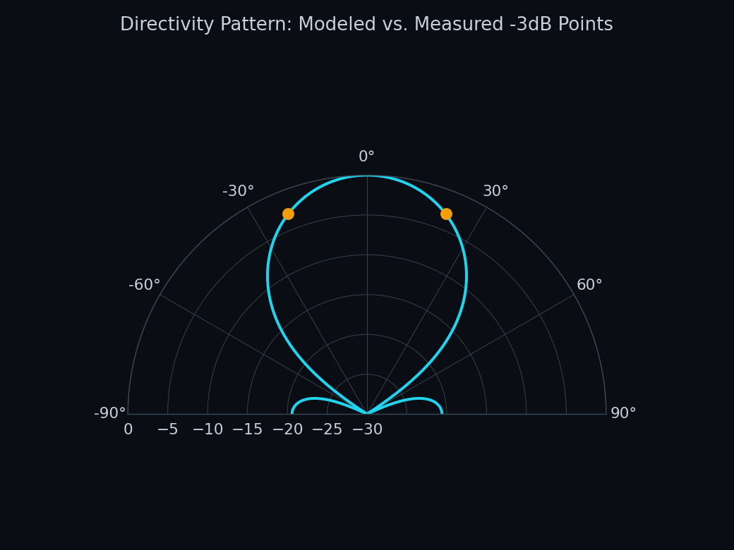
Because the effective radius was solved specifically so that the model reproduces the measured beam width, that match is a property of the fit rather than a second independent confirmation. What the fit does show is that the required radius is physically reasonable: about 26 mm, giving a 52 mm effective diameter, a sensible size for this transducer's actual radiating face, not an arbitrary number a curve fit happened to produce. Combined with the visual match to the measured pattern's overall shape in Figure 20, not just the single calibration point, this is consistent with the transducer behaving, to first order, as a circular piston radiator without invoking higher-order vibration modes.
6. Time-Frequency Signal Analysis
A 1 kHz, 1 Vpp sine reference signal was captured via TopView2000 at five different timebase settings
(200 Hz, 500 Hz, 1 kHz, 2 kHz, and 5 kHz) to demonstrate the practical consequence of the Nyquist-Shannon
sampling theorem on waveform reconstruction fidelity, then analyzed by FFT to examine how the sampling
timebase and record length shape the resulting frequency-domain spectrum. The original analysis (matlab605.m)
computed abs(fft(signal)) for the 5 kHz record and plotted it directly against sample index,
reproduced in Figure 21.
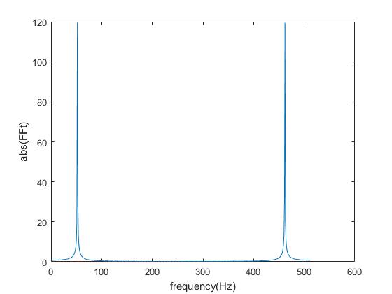
Figure 22 extends that same computation, unchanged, to all five real time-domain records captured in this experiment, using each record's own real sample interval to build a properly scaled frequency axis, then stacks the five spectra into one three dimensional waterfall so they can be compared directly instead of one at a time.
Raw data captured
1khz 1VPP.txt · 200hz 1VPP.txt · 2khz 1VPP.txt ·
500hz 1VPP.txt · 5khz 1VPP.txt · 5khz Time.txt · 5khz FFT.txt
7. Derived Performance Metrics & Industry Relevance
Sections 3 through 5 report what was measured. This section derives, from that same raw data, the three numbers a working sonar or ultrasonic transducer engineer would actually want: how efficiently it converts electrical drive into mechanical motion, how sharply it resonates, and how much usable bandwidth it has. Every value below is computed directly from the frequency/conductance/susceptance records behind Figures 4 through 11 and from the TVR record behind Figure 14, not looked up or assumed.
7.1 Electromechanical Coupling Coefficient (k_eff)
The effective electromechanical coupling coefficient follows directly from the series resonance Fs and the antiresonance Fp already marked in Figures 5, 7, 9, and 11, via the standard IEEE resonance-method formula:
| Condition | Fs (kHz) | Fp (kHz) | k_eff (derived here) | Instrument-reported Keff |
|---|---|---|---|---|
| Hydrophone, air | 112.30 | 123.70 | 0.4193 | 0.4193 |
| Hydrophone, water | 112.30 | 123.75 | 0.4201 | 0.4201 |
| Transducer, air | 38.68 | 41.14 | 0.3406 | 0.3406 |
| Transducer, water | 39.28 | 42.00 | 0.3540 | 0.3540 |
All four measurement screenshots in Section 3 print the instrument's own Keff reading in the corner of the plot (Figures 4, 6, 8, and 10). The value derived here independently from the raw Fs/Fp pair, using nothing but the standard formula above, matches the instrument's own reading to four decimal places in all four conditions, validating both the raw data export and the formula before either is relied on elsewhere in this report.
Industry relevance. The electromechanical coupling coefficient is one of the headline specification numbers on every commercial piezoceramic and sonar-transducer datasheet. It is used for material and design screening (a higher k converts more of the electrical drive into useful motion and supports wider usable bandwidth), for incoming-inspection quality control (a resonance/antiresonance sweep like the one used here is a standard production-line acceptance test for piezo elements), and for predicting how much drive energy stays trapped as reactive electrical energy versus how much actually leaves the device as sound or motion.
7.2 Mechanical Quality Factor (Qm)
The mechanical quality factor is computed from the same conductance curve using the standard half-power (−3 dB) bandwidth method: Qm = Fs / (F2 − F1), where F1 and F2 are the frequencies on either side of Fs at which conductance falls to Gmax/√2.
| Condition | Fs (kHz) | F1 (kHz) | F2 (kHz) | Qm (−3 dB, derived here) | Qm (instrument-reported) |
|---|---|---|---|---|---|
| Hydrophone, air | 112.30 | 110.55 | 113.95 | 33.03 | 20.68 |
| Hydrophone, water | 112.30 | 110.60 | 114.00 | 33.03 | 20.51 |
| Transducer, air | 38.68 | 38.56 | 38.82 | 148.77 | 89.70 |
| Transducer, water | 39.28 | 38.40 | 40.08 | 23.38 | 14.41 |
The instrument's own on-screen Qm is consistently lower than the value derived here, by close to the same factor (about 0.6×) in all four conditions. Fs, Fp, and k_eff all matched the instrument exactly in Section 7.1, so this is not a data error; it means the instrument's built-in Qm uses a different, wider bandwidth convention than the IEEE half-power (Gmax/√2) method used here, and the two are not directly comparable in absolute terms. What both methods agree on, using either convention, is the same conclusion below.
By the −3 dB definition used in this report, the transducer's Qm collapses from about 149 in air to about 23 in water, a drop of roughly a factor of 6; by the instrument's own convention it collapses from about 90 to about 14, a drop of roughly a factor of 6 as well. This is exactly the expected signature of radiation loading: once the piston face couples to water, acoustic power radiated away damps the mechanical resonance and broadens it, and both bandwidth conventions see the same effect by the same proportion. The hydrophone, by contrast, barely changes under either convention (about 33 versus 33 here, about 21 versus 21 on the instrument), consistent with it being a much smaller, lighter, receive-only element whose resonance is dominated by its own structure rather than by radiation loading.
Industry relevance. Qm sets the sensitivity/bandwidth tradeoff. High-Q resonant designs (fish-finder and depth-sounder transducers, for example) concentrate sensitivity into a narrow band; low-Q broadband designs (communication and wideband imaging sonar transducers) sacrifice peak sensitivity for usable bandwidth. Qm is also used to predict self-heating under continuous drive and to design the electrical matching network that keeps a transducer looking resistive to its driving amplifier near resonance.
7.3 Acoustic Bandwidth from the TVR Curve
The same −3 dB method applied directly to the measured TVR curve of Figure 14 gives an independent, purely acoustic bandwidth and quality factor for the transducer while it is actually radiating into water:
This acoustic Q (13.3) sits much closer to the water-loaded electrical Qm from Section 7.2 (23.4) than to the air value (148.8), which makes physical sense: the TVR sweep and the water-immersed impedance sweep are both measuring the same radiation-loaded transducer, just through two different instruments (an acoustic output measurement in Section 5 and an electrical impedance sweep in Section 3). Two independent experiments in this report agree on the same underlying physics.
Industry relevance. Usable bandwidth determines what a transducer can actually do downstream: wide bandwidth is required for pulse-compression and chirp sonar waveforms and for high-resolution ranging, while narrow bandwidth concentrates available drive power into a single frequency for maximum range at that frequency. The tradeoff visible here (very high on-axis output, only about 3 kHz of usable bandwidth) is exactly why practical broadband sonar transducers usually need multiple resonant elements or a deliberately engineered wideband matching network rather than a single simple resonator.
7.4 Summary
| Parameter | Value | Reference |
|---|---|---|
| Hydrophone series resonance Fs | 112.30 kHz | Figures 4, 6 |
| Hydrophone antiresonance Fp | 123.70 to 123.75 kHz | Figures 5, 7 |
| Hydrophone k_eff | 0.419 to 0.420 | Section 7.1 |
| Transducer series resonance Fs (air / water) | 38.68 / 39.28 kHz | Figures 8, 10 |
| Transducer k_eff (air / water) | 0.341 / 0.354 | Section 7.1 |
| Transducer Qm (air / water) | 148.8 / 23.4 | Section 7.2 |
| TVR peak level (at 39.8 kHz) | 225.7 dB | Figure 14 |
| TVR −3 dB bandwidth / acoustic Q | 3.0 kHz / 13.3 | Section 7.3 |
| Measured beam width (−3 dB, 39.8 kHz) | 42.99° | Section 5.2 |
| Directivity factor / index | 8.058 / 9.06 dB | Section 5.2 |
| Effective piston radius / diameter (fitted) | 26.1 mm / 52.2 mm | Section 5.3 |
8. Conclusion & Design Implications
Across impedance, sensitivity, transmitting response, and directivity, the measured behavior of the test transducer is internally consistent: the impedance and sensitivity curves both identify a resonance near 39.3 to 39.8 kHz, the transmitting response peaks in the same band (Figures 14 and 15), and the measured directivity pattern at that same frequency is well described by a circular-piston diffraction model calibrated to reproduce the measured beam width, yielding a physically reasonable 52 mm effective radiating diameter rather than an arbitrary fitting parameter (Figures 16 through 20). The derived metrics in Section 7 add an independent line of evidence: the electromechanical coupling coefficient computed from the raw impedance data matches the instrument's own reading in all four measured conditions, and the transducer's mechanical Q collapses by roughly a factor of 6 in water under either bandwidth convention, a drop the independently measured acoustic bandwidth in Section 7.3 lands in the same neighborhood of, since both are responding to the same radiation-loading physics. That agreement between two different instruments measuring two different quantities is itself a useful design check: it confirms the transducer is operating in its fundamental piston mode rather than exciting spurious higher-order face vibrations, and it means the calibrated model can be used with reasonable confidence to predict performance at other frequencies or ranges before committing to a full 3D FEM study in COMSOL or an equivalent piezoelectric solver.